Chapter 3 Running Bayesian models
Different software and R packages can be used to run Bayesian models. Whether it is a LCM or a more conventional regression model is not very important at this stage. In this document we will use a software called JAGS and the R2jags package. So, if not already done, you will have to download JAGS here and install it on your computer.
Basically, to run any Bayesian model, we will always need the same three things:
- Data
- A model containing:
- A likelihood function linking observed data to unknown parameters
- A prior distribution for each unknown parameter
- An initial value for each unknown parameter to start the Markov chains
- These values can also be generated randomly by the software, but specifying them will improve reproducibility
3.1 The data
This is the easy part. If we were to run, for instance, a “conventional” regression analysis, we would have to import in R a complete dataset (e.g., a CSV file) with a row for each observation and a column for each variable. However, when using LCM to estimate disease prevalence or diagnostic accuracy, the dataset is simply the number of individuals in each category. For instance, to estimate a simple prevalence (Prev), we could have 30 individuals that tested positive (variable T) out of a total of 100 individuals (variable n). In such case, the dataset could be created as follow:
If we want to check that it works, we could ask to see this new R object.
## $T
## [1] 30
##
## $n
## [1] 100
3.2 The model
3.2.1 The likelihood function
Let’s start with a simple example, estimating a single proportion. For estimating a proportion we could describe the likelihood function linking unknown parameters to observed data as follows:
\(T \sim dbin(Prev, n)\)
In other words: the disease prevalence (Prev), an unknown parameter, can be linked to the observed number of positive individuals (T) and the total number of tested individual (n) through the binomial function.
In this case, the values of T and n are the observed data and Prev is the only unknown parameter.
3.2.2 Priors for unkown parameters
We will have to specify a prior distribution for each unknown parameter (using the \(\sim\) sign).
In the preceding example, we only have one unkown parameter, Prev, which is a proportion. Theoretically such parameter could take values from 0 to 1, so a beta distribution would be one way to describe its prior distribution. We could use the epi.betabuster() function from the epiR library to define a given beta distribution based on previous knowledge, as described in the previous sections. Moreover, if we want to use a flat prior, we could simply choose the value 1.0 for the a and b shape parameters.
In the following code, I am creating R objects for a and b for Prev beta prior distributions.
With informative priors, for instance, if we know from the literature that the prevalence is expected to be 0.25 with 95CI of (0.20, 0.30), we could instead use the following code and assign these values to Prev.shapea and Prev.shapeb:
library(epiR)

# Prevalence as Mode=0.25, and we are 97.5% sure <0.30
rval <- epi.betabuster(mode=0.25,
                       conf=0.975,
                       imsure="less than",
                       x=0.30)

rval$shape1                #View the a shape parameter in rval
## [1] 81.872## [1] 243.616#The two lines below would be used to assign the generated values for later usage. Below we decided to rename this parameters Prev.shapea and Prev.shapeb since they will represent the a and b shape parameters for the Beta distribution describing the disease prevalence
Prev.shapea <- rval$shape1
Prev.shapeb <- rval$shape23.2.3 Creating the JAGS model
Our Bayesian model has to be presented to JAGS as a text file (i.e., a .txt document). To create this text file, we will use the paste0() function to write down the model and then the write.table() function to save it as a .txt file.
An interesting feature of the paste0() function is the possibility to include R objects in the text. For instance, we may want to have a generic model that will not be modified, but within which we would like to change the values used to describe the priors. We could include these “external” values within our paste0() function. Thus, we just have to change the value of the R object that our model is using, rather than rewriting a new model. In the previous section, we created two R objects called Prev.shapea and Prev.shapeb (which were the a and b shape parameters for the prior distribution of our proportion Prev). To describe our prior distribution, we can ignore this previous work that we have done and directly create a short text as follows:
text1 <- paste0("Prev ~ dbeta(1, 1)")       #Creating a short text named "text1"
text1                                       #Asking to see the text1 object
## [1] "Prev ~ dbeta(1, 1)"However, if the same model is to be applied later with a different prior distribution, it may be more convenient to leave the a and b shape parameters as R objects. Thus, if we change the prior distribution and run the script again, we would run the entire analyses with the newly created distribution. For instance, the code below would use the a and b shape parameters that we created above.
text2 <- paste0("Prev ~ dbeta(",Prev.shapea,", ",Prev.shapeb,")")            #Creating a short text named "text2" and containing other already created R objects
text2                                                                        #Asking to see the text2 object
## [1] "Prev ~ dbeta(81.872, 243.616)"When using paste0(), any text appearing outside of sets of quotation marks (e.g., Prev.shapea and Prev.shapeb in the preceding script) will be considered as R objects that need to be included in the text. Thus, later, we could just change the values for Prev.shapea and Prev.shapeb and our model will be automatically modified.
Some important notes about the text file containing the model before we start with R2jags:
JAGS is expecting to see the word “model” followed by curly brackets { }. The curly brackets will contain the likelihood function AND the priors.
Similarly to
R, any line starting with a # will be ignored (these are comments).Similarly to
R, <- means equal.The ~ symbol means “follows a distribution”.
Similarly to
R,JAGSis case sensitive (i.e., P does not equal p).Loops can be used with keyword “for” followed by curly brackets.
Array can be indicated using squared brackets [ ].
In the example below, we create an R object called model_single_prop using the paste0() function and then save it as a text file using the write.table() function. We will check this text file below and then explain the code for the model.
# Specify the model
model_single_prop <- paste0("model{

#=== LIKELIHOOD ===#

  T ~ dbin(Prev, n)


#=== PRIOR  ===#

  Prev ~ dbeta(",Prev.shapea,", ",Prev.shapeb,")    ## Prior for Prev

}")

#write as a text (.txt) file
write.table(model_single_prop,
            file="model_single_prop.txt",
            quote=FALSE,
            sep="",
            row.names=FALSE,
            col.names=FALSE)
Here is a snapshot of the final result (i.e., the text file):
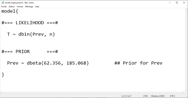
In the preceding script, the paste0() function was used to create the text, as an R object, that will be needed for the .txt file. This text is mainly “static”, except for the a and b parameters of the beta distribution used to describe our prior knowledge on disease prevalence. We can see that, if we were to modify and then run the preceding script where we assigned values to these parameters, and then run again the paste0() function, our text file would be updated with new values for our prior distribution. This is a feature that we will use a lot, especially with more complex LCM, to minimize the amount of work and the risk of typographic errors..
The write.table() function was simply used to save, as a .txt file, the R object containing the text we just created.
Both the paste0() and write.table() functions are part of basic R, no need to install or call a given library.
3.3 Generating initial values
The initial value is the first value where each Markov chain will start.
- We have to specify one initial value for each unknown parameter in the model.
- If we decide to run three Markov chains, we will need three different sets of initial values.
- We can also let the software choose a random value to start each chain, but it will then be impossible to exactly reproduce a given result. For instance, if we have obtained a very awkward Markov chain, we may not be able to reproduce this result to investigate what went wrong. Note, though, that it would be quite uncommon for a Markov chain to be extremely “sensitive” to the chosen starting value. But we will see during the workshop that it will sometimes happen.
In our preceding example we have one unknown parameter (Prev). If we were to run three Markov chains, we could generate three sets of initial values for this parameter as follows. Of course, the chosen values could be changed. In the case of a proportion, we can specify any value between 0 and 1.
#Initializing values for the parameter "Prev" for the 3 chains
inits <- list(
  list(Prev=0.10),
  list(Prev=0.50),
  list(Prev=0.90)
  )
We now have an R object called inits that contains the three values where each Markov chains will start.
3.4 Running a model in JAGS
We now have the three elements that we needed: the data, the model, and a set of initial values. We can now use the R2jags library to run our Bayesian analysis. The R2jags package provides an interface from R to the JAGS software for Bayesian data analysis. JAGS uses Markov Chain Monte Carlo (MCMC) simulation to generate a sample from the posterior distribution of the parameters.
The R2jags function that we will use for that purpose is the jags() function. Here are the arguments that we need to specify:
- The dataset using
data=
- The text file containing the model written in
JAGScode usingmodel.file=
- The names of the parameters which should be monitored using
parameters.to.save=
- The number of Markov chains using
n.chains=. The default is 3
- The sets of initial values using
inits=. If inits is NULL,JAGSwill randomly generate values
- The number of total iterations per chain (including burn-in; default: 2000) using
n.iter= - The length of burn-in (i.e., number of iterations to discard at the beginning) using
n.burnin= - The thinning rate, which represent how many of the values sampled by the MCMC will be retained. The default is 5 (1 out of 5). Since there is no a priori need for thinning, we can specify
n.thin=1 in most situations - The last argument
DIC=TRUEorDIC=FALSEwill determine whether to compute the deviance, pD, and deviance information criteria (DIC). These could sometimes be useful for model selection/comparison. We could leave that toDIC=FALSEsince we will not be using these values during the workshop
With the following code, we will create an R object named bug.out. This object will contain the results of running our model with the specified priors using the available data, and the sets of initial values that we have created. For this analysis, we have asked to run 3 Markov chains for 6000 iterations each and we discarded the first 1000 iterations of each chain. Finally, we will monitor our only unknown parameter: Prev.
library(R2jags)
library(coda)

#Run the Bayesian model
bug.out <- jags(data=datalist,                             #Specifying the R object containing the data
               model.file="model_single_prop.txt",         #Specifying the .txt file containing the model
               parameters.to.save=c("Prev"),               #Specifying the parameters to monitor. When >1 parameter, it will be a list, ex: c("Prev", "Se", "Sp")
               n.chains=3,                                 #Number of chains
               inits=inits,                                #Specifying the R object containing the initial values
               n.iter=6000,                                #Specifying the number of iterations
               n.burnin=1000,                              #Specifying the number of iterations to remove at the beginning
               n.thin=1,                                   #Specifying the thinning rate
               DIC=FALSE)                                  #Indicating that we do not request the deviance, pD, nor DIC
## Compiling model graph
## Resolving undeclared variables
## Allocating nodes
## Graph information:
## Observed stochastic nodes: 1
## Unobserved stochastic nodes: 1
## Total graph size: 5
##
## Initializing modelAs we can see, we received a few messages. It looks good, don’t you think?
3.5 Model diagnostic
Before jumping to the results, we should first verify that:
- The chains have converged,
- The burn-in period was long enough,
- We have a sample of values large enough to describe the posterior distribution with sufficient precision,
- The Markov chains behaved well (mainly their auto-correlation).
There are many diagnostic methods available for Bayesian analyses, but, for this workshop, we will mainly use basic methods relying on plots.
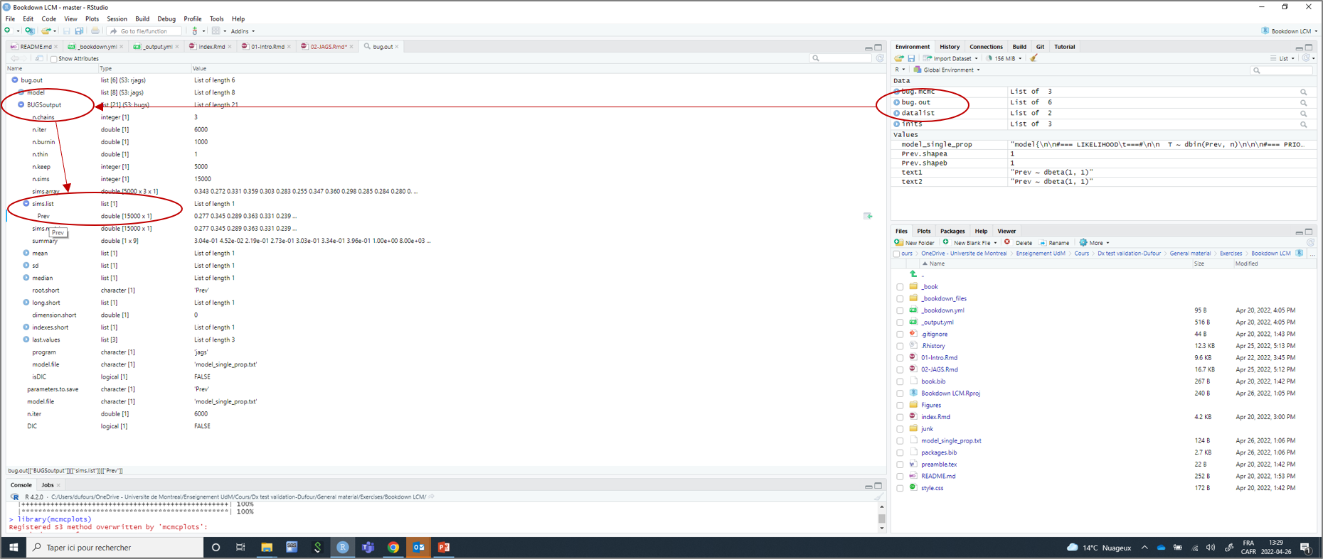
Diagnostics are available when we convert our model output into a MCMC object using the as.mcmc() function of the mcmcplots library.
library(mcmcplots)
bug.mcmc <- as.mcmc(bug.out)          #Converting the model output into a MCMC object (for diagnostic plots)
Then, we can apply the mcmcplot() function on this newly created MCMC object.
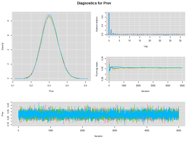
When we do that, a HTML document will be created and our web browser will automatically open it. Here is a snapshot of the HTML file in our browser:
3.5.1 Convergence and burn-in
To check whether convergence of the Markov chains was achieved we can inspect the “trace plot” (the bottom figure) presenting the values that were picked by each chain on each iteration. The different chains that we used (three in the preceding example) will be overlaid on the trace plot. We should inspect the trace plot to evaluate whether the different chains all converged in the same area. If so, after a number of iterations they should be moving in a relatively restricted area and this area should be the same for all chains.
The plots above would be a good example of the trace plot of three “nice” Markov chains (lucky us!). In this preceding example, we can see on the trace plot that the chains had already converged (probably way before the end of the first 1000 iterations that were excluded) toward the same area. On the trace plot, we can only see the values that were stored after the burn-in period. The chains were then moving freely within this limited area (thus sampling from the posterior distribution).
We could conclude based on the trace plot that:
- The Markov chains did converge
- A short burn-in period of less than a 1000 iterations would have been sufficient. Note that we will often use a longer burn-in (e.g., 5,000 or even more) just to be sure and because it only costs a few more seconds on our computer…
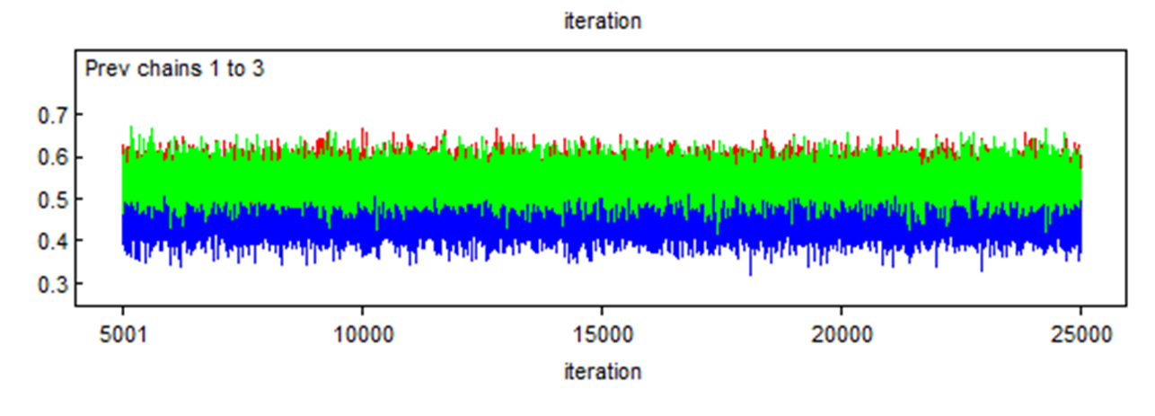
Here is another example where two chains (the red and green) converged in the same area, but a third one (the blue) also converged, but in a different area. We should be worried in such case. We will see later the reason for such behavior.
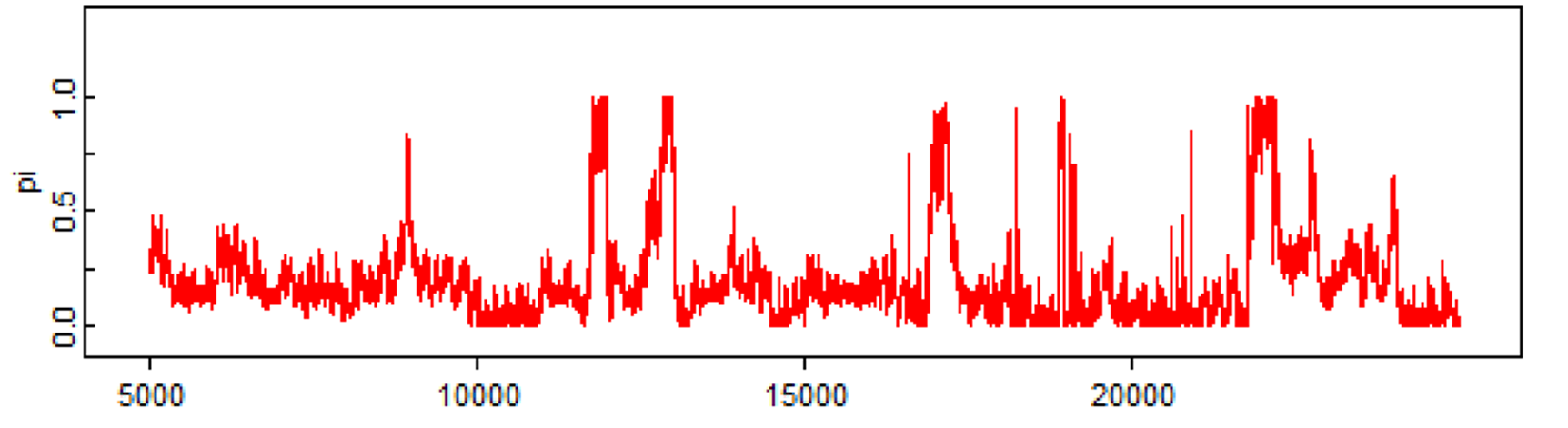
Finally, here is a last example with just one Markov chain which clearly did not converge, even after 25,000 iterations. We should be terrified by that!!! ;-).
3.5.2 Number of iterations
Next, we can inspect the posterior distributions to determine if we have a large enough sample of independent values to describe with precision the median estimate and the 2.5th and 97.5th percentiles. The effective sample size (EES) takes into account the number of values generated by the Markov chains AND whether these values were auto-correlated, to compute the number of “effective” independent values that are used to describe the posterior distribution. Chains that are auto-correlated will generate a smaller number of “effective values” than chains that are not auto-correlated.
The effectiveSize() function of the coda library provide a way to appraise whether we had enough iterations. In the current example, we already created a mcmc object named bug.mcmc. We can ask for the effective sample size as follows:
##     Prev
## 8991.268
So we see here that, despite having stored 3 times 5,000 values (15,000 values), we have the equivalent of roughly 10,000 independent values. What to do with this information? Well, we could, for instance, decide on an arbitrary rule for ESS (say 10,000 values) and then adapt the length of the chains to achieve such an ESS for each of the selected parameters, because the effective sample sizes will not be the same for all parameters.
3.5.3 Auto-correlation
Remember that a feature of Markov chains is to have some auto-correlation between two immediately subsequent iterations, and then a correlation that quickly goes down to zero (i.e., they have a short memory). The auto-correlation plot can be used to assess if this feature is respected.
From our previous example (check the upper right figure in the plot below), it seems that it is the case.
Here is another example where we do have an auto-correlation that is persisting.
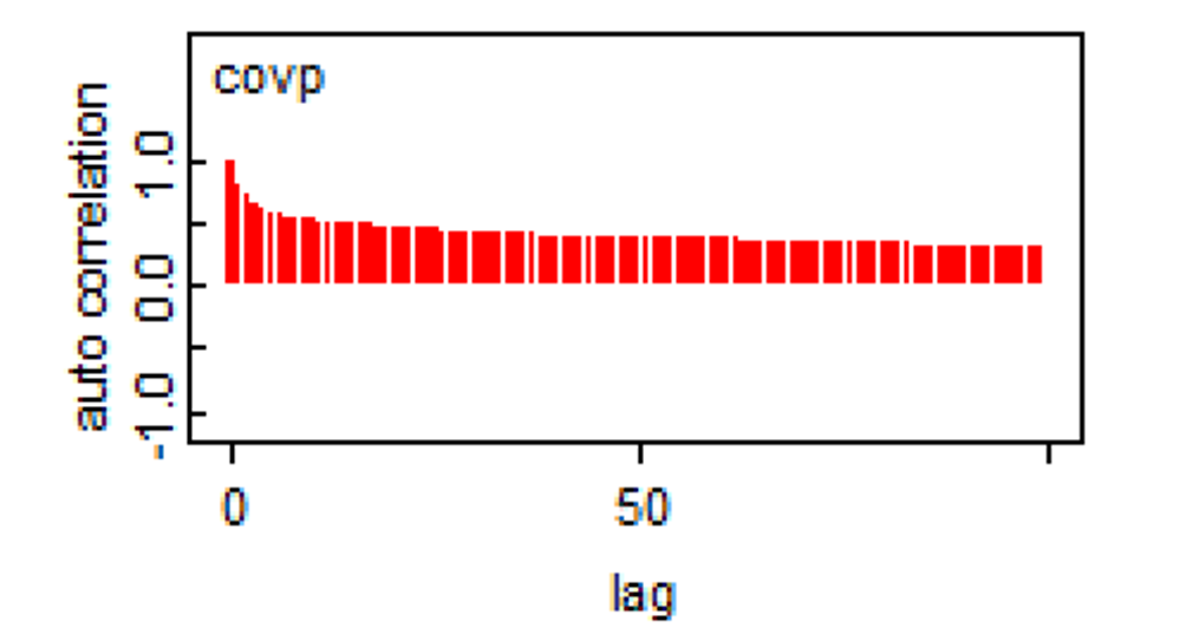
When such a behavior is observed, running the chains for more iterations will help achieve the desire ESS. In some situations, specifying different priors (i.e., increasing the amount of information in priors) may also help. In the past, thinning of the Markov chains (i.e., discarding all but every kth sampled value) was often used when autocorrelation was detected, but this method is not recommended anymore, except for rare instances where computer memory limitations would be a problem Link et Eaton, 2012.
3.6 Getting our estimates
Now, if we are happy with the behavior of our Markov chains, the number of iterations, and burn-in period, we can summarize our results (i.e., report the median, 2.5th and 97.5th percentiles) very easily with the print() function. Below, we also indicated digits.summary=3 to adjust the precision of the estimates that are reported (the default is 1).
print(bug.out,                  #Asking to see the mean, median, etc of the unknown parameters that were monitored
      digits.summary=3)         #Requiring a precision of 3 digits
## Inference for Bugs model at "model_single_prop.txt", fit using jags,
## 3 chains, each with 6000 iterations (first 1000 discarded)
## n.sims = 15000 iterations saved. Running time = 0.81 secs
## mu.vect sd.vect 2.5% 25% 50% 75% 97.5% Rhat n.eff
## Prev 0.263 0.021 0.221 0.248 0.262 0.277 0.305 1.001 15000
##
## For each parameter, n.eff is a crude measure of effective sample size,
## and Rhat is the potential scale reduction factor (at convergence, Rhat=1).Here we see that the median Prev estimate (95BCI) was 26% (22, 31).
We can also plot the bug.mcmc object that we have created using the plot() function to produce the trace plot and a density plot presenting the posterior distributions of each unknown parameter.
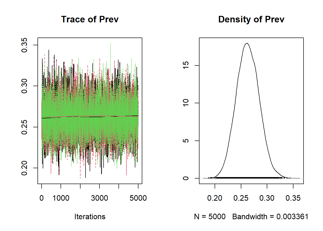
Figure 3.1: Trace plot and density plot produced using the plot() function.
If we prefer to work on our own plots, note that all the values sampled from our posterior distributions were stored in the bug.out object that we have created. If we inspect the bug.out object, we will notice an element named BUGSoutput, inside this element, there is another object named sims.list, within this sims.list, there is an element named Prev. As we can see below, this element is made of a list of 15,000 values. This correspond to the 5,000 values sampled (1/iteration) by each Markov chain (3 chains) for the unknown parameter Prev. So this element is simply all the sampled values assembled together.
We could use this element, for instance, to plot together the prior and posterior distributions on a same figure. On the figure below, the prior distribution is not obvious, it is the flat dashed red line just above the x axis (remember, we used a flat prior for Prev).
#Plot the posterior distribution
plot(density(x=bug.out$BUGSoutput$sims.list$Prev),      #Indicating variable to plot
     main="Disease prevalence",                         #Title for the plot
     xlab="Prevalence", ylab="Density",                 #x and y axis titles
     )

#plot the prior distribution
curve(dbeta(x,
            shape1=Prev.shapea,
            shape2=Prev.shapeb),
      from=0, to=1,
      lty=2,                    #Asking for a dashed line pattern
      col="red",                #Asking for a red line
      add=TRUE)                #Asking to add this plot to the preceding one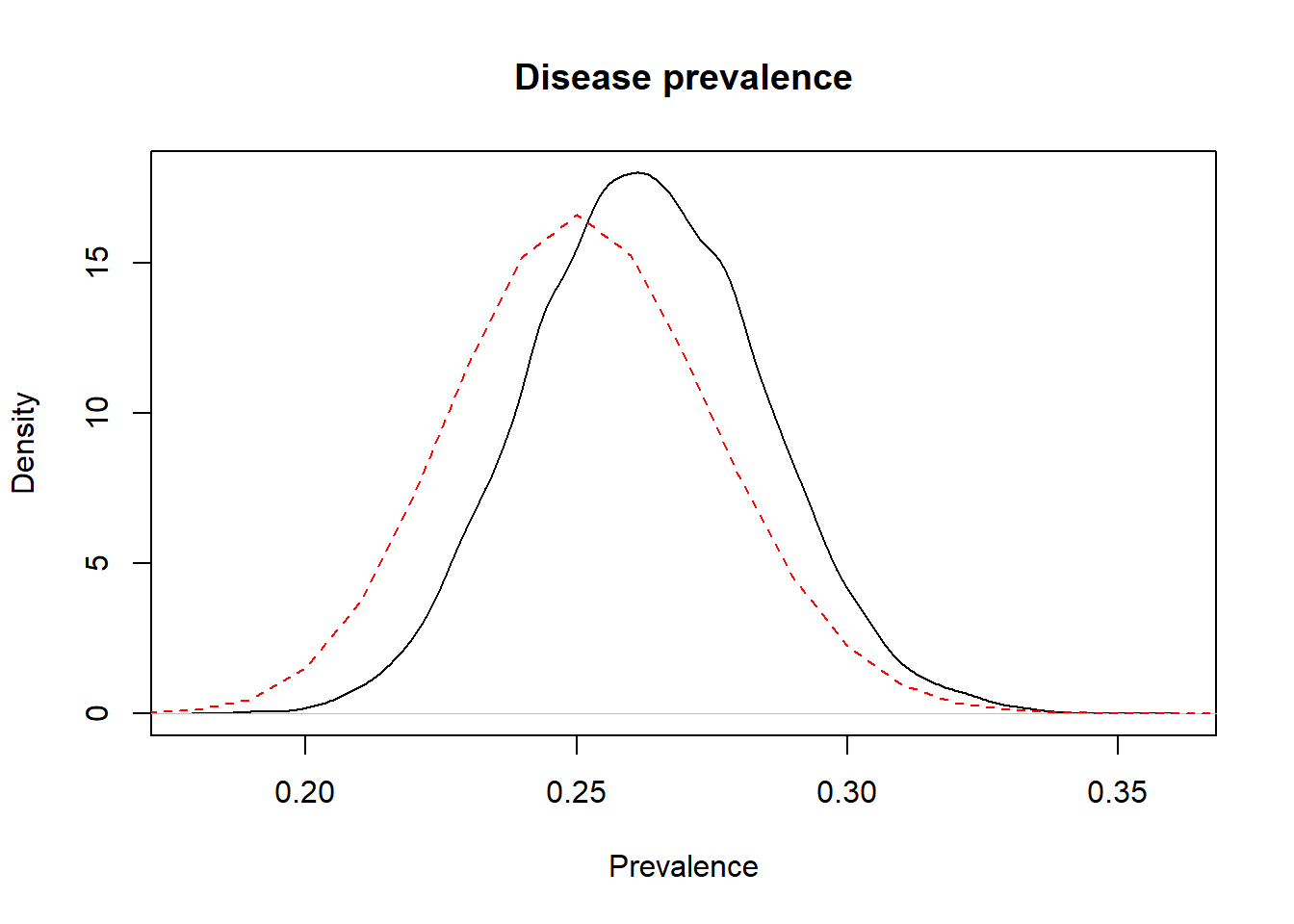
Figure 3.2: Prior (dashed red line) and posterior (full black line) distribution of the prevalence of disease.